Plotting the distribution of floating point numbers
There is an interesting post from 2010
that plotted the distribution of a custom 6-bit floating point format. I was curious what the resulting graph would
look like if we plotted IEEE single precision floating point numbers, instead. Luckily, this turns out to be
very easy using the gnuplot utility!
The trick is to use the nextafterf (manpage) function to create an enumeration
of the floating point numbers. There are too many floating point numbers to plot every single one, so we'll arbitrarily
choose to only plot every hundred-thousandth floating point number, counting up to the hundred-millionth
floating point number. We'll do this in both the positive and negative directions.
Here is the code we'll use to generate the data.txt file for gnuplot to plot from. All we need
to do is generate a text file with two space-delimited columns. The first column will hold the
current index during iteration, and the second column will hold the decimal approximation of the
floating point number.
#include <float.h>
#include <math.h>
#include <stdbool.h>
#include <stdio.h>
#include <stdlib.h>

#define INDEX_MAX (100 * 1000 * 1000)
// Plotting every single floating point number would bloat the
// data file way too much. Let's only plot every floating point
// number in steps of INDEX_STEP.
#define INDEX_STEP (100 * 1000)

int main(void) {
  FILE *file = fopen("data.txt", "w");
  if (!file) {
    perror("Failed to open 'data.txt' for writing");
    exit(EXIT_FAILURE);
  }

  // Plotting positive numbers
  int index = 0;
  float current = 0.0f;
  while (index <= INDEX_MAX && current != HUGE_VALF) {
    bool should_print = index % INDEX_STEP == 0;
    if (should_print &&
        fprintf(file, "%d %.*g\n", index, FLT_DECIMAL_DIG, current) < 0) {
      perror("Failed to write to 'data.txt'");
      exit(EXIT_FAILURE);
    }
    current = nextafterf(current, FLT_MAX);
    index += 1;
  }

  // Plotting negative numbers
  index = 0;
  current = 0.0f;
  while (index <= INDEX_MAX && current != HUGE_VALF) {
    bool should_print = index % INDEX_STEP == 0;
    if (should_print &&
        fprintf(file, "-%d %.*g\n", index, FLT_DECIMAL_DIG, current) < 0) {
      perror("Failed to write to 'data.txt'");
      exit(EXIT_FAILURE);
    }
    current = nextafterf(current, -FLT_MAX);
    index += 1;
  }

  exit(EXIT_SUCCESS);
}
What is FLT_DECIMAL_DIG in the code?
Approximately paraphrasing the C23 standard (PDF), it gives us the number of digits we need to write a single precision floating point number in decimal form such that it can be converted back into the exact same floating point number. The decimal form is not exact, but since we can map the decimal back to precisely one floating point number, it's good enough for this graphing exercise.
Thanks to this stack overflow post which taught me about this macro.
After running this code, we can generate the graph using the following gnuplot script:
set title "Enumeration of Floating Point Numbers using nextafterf()" font ",18" offset 0,1
set xlabel "Index during iteration (negative values represent iteration towards -FLT\\\_MAX)" font ",11" offset 0,-2
set ylabel "Approximate value of nextafterf() at index" offset -4,0 font ",11"
unset key
set xtics axis
set ytics axis
set zeroaxis
set margin 12,12,5,5
unset border
set xtics -1e8,2e7,1e8

plot "data.txt" lc 2
pause -1 "Hit any key to continue"
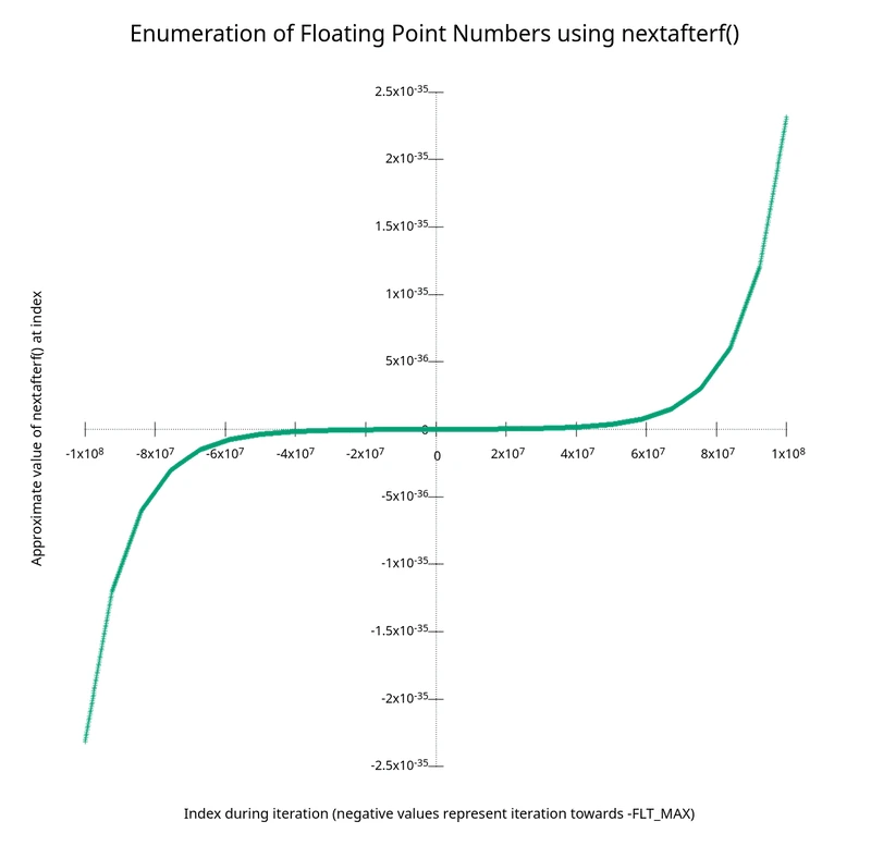
Putting it all together, we get the following image:

With the accompanying table giving the coordinates of key points on the graph if you're curious. Note that, as
mentioned in the graph, the negative values in the "Index during iteration" column represent iterations towards -FLT_MAX):
| Index during iteration | Approximate value of nextafterf() at index |
|---|---|
| -1×10⁸ | -2.31223412×10⁻³⁵ |
| -8×10⁷ | -4.62446824×10-36 |
| -6×10⁷ | -8.67087796×10-37 |
| -4×10⁷ | -1.66296864×10-37 |
| -2×10⁷ | -3.25420516×10-38 |
| 0 | 0 |
| 2×10⁷ | 3.25420516×10-38 |
| 4×10⁷ | 1.66296864×10-37 |
| 6×10⁷ | 8.67087796×10-37 |
| 8×10⁷ | 4.62446824×10-36 |
| 1×10⁸ | 2.31223412×10⁻³⁵ |
The most interesting part of this data is that we can notice the gaps get bigger between the points the farther away we get from zero! This makes sense, as incrementing the last bit in the fractional part of a floating point number (which is basically what takes us to the next floating point number) gives us a larger and larger difference as the exponent for the number grows.